Note
Go to the end to download the full example code.
1. Exploratory Data Analysis
In this file we analyze the data using some basic statistics and exploratory plots. The purpose is to get familiarize with the data
synthesis time: hydrothermal reaction time (time taken to prepare the material)
band gap: property of material (how much energy is required to excite one electron from outermost shell)
volume : volume of wastewater
import numpy as np

import matplotlib as mpl
import matplotlib.pyplot as plt
import pandas as pd

from sklearn.manifold import TSNE

from easy_mpl import boxplot, pie
from easy_mpl.utils import create_subplots, despine_axes, map_array_to_cmap

from utils import CATEGORIES
from utils import set_rcParams
from utils import SAVE, version_info
from utils import read_data, LABEL_MAP, plot_correlation, prepare_data
/home/docs/checkouts/readthedocs.org/user_builds/weil101/envs/latest/lib/python3.12/site-packages/sklearn/experimental/enable_hist_gradient_boosting.py:15: UserWarning: Since version 1.0, it is not needed to import enable_hist_gradient_boosting anymore. HistGradientBoostingClassifier and HistGradientBoostingRegressor are now stable and can be normally imported from sklearn.ensemble.
  warnings.warn(
/home/docs/checkouts/readthedocs.org/user_builds/weil101/envs/latest/lib/python3.12/site-packages/ai4water/datasets/__init__.py:3: UserWarning: datasets module is deprecated. Please install aqua-fetch using
              pip install aqua-fetch
              and import corresponding dataset from there.
  warnings.warn("""datasets module is deprecated. Please install aqua-fetch using

**********Tensorflow models could not be imported **********
for lib, ver in version_info().items():
    print(lib, ver)
python 3.12.10 (main, May  6 2025, 10:49:23) [GCC 11.4.0]
os posix
ai4water 1.07
lightgbm 4.6.0
catboost 1.2.10
xgboost 3.2.0
easy_mpl 0.21.5
SeqMetrics 2.0.0
numpy 1.26.4
pandas 2.2.3
matplotlib 3.10.8
h5py 3.16.0
sklearn 1.3.1
optuna 4.8.0
skopt 0.10.2
plotly 6.6.0
seaborn 0.13.2
crepes 0.9.0
mapie 0.9.2
shap 0.49.1
scipy 1.17.1
set_rcParams()
data = read_data(outputs=['k', 'Efficiency'])
printing number of rows and number of columns in the data
print(data.shape)
(1527, 36)
printing counts of missing values
data.isna().sum()
Catalyst                             0
Hydrothermal synthesis time (min)    0
Energy Band gap (Eg) eV              0
C (At%)                              0
O (At%)                              0
Fe (At%)                             0
Al (At%)                             0
Ni (At%)                             0
Mo (At%)                             0
S (At%)                              0
Bi                                   0
Ag                                   0
Pd                                   0
Pt                                   0
Surface area (m2/g)                  0
Pore volume (cm3/g)                  0
Pore size (nm)                       0
volume (L)                           0
loading (g)                          0
Light intensity (watt)               0
Light source distance (cm)           0
Time (m)                             0
Dye                                  0
log_Kw                               0
hydrogen_bonding_acceptor_count      0
hydrogen_bonding_donor_count         0
solubility (g/L)                     0
molecular_wt (g/mol)                 0
pka1                                 0
pka2                                 0
Dye concentration (mg/L)             0
Solution pH                          0
HA (mg/L)                            0
Anions                               0
k                                    0
Efficiency                           0
dtype: int64
data.describe()
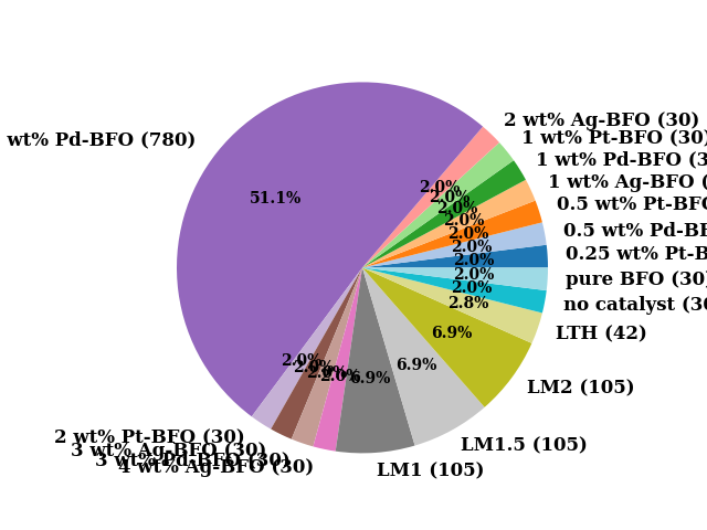
print(len(data['Catalyst'].unique()))

data['Catalyst'].unique()
18

array(['LTH', 'LM1', 'LM1.5', 'LM2', 'no catalyst', 'pure BFO',
       '0.5 wt% Pd-BFO', '1 wt% Pd-BFO', '2 wt% Pd-BFO', '3 wt% Pd-BFO',
       '1 wt% Ag-BFO', '2 wt% Ag-BFO', '3 wt% Ag-BFO', '4 wt% Ag-BFO',
       '0.25 wt% Pt-BFO', '0.5 wt% Pt-BFO', '1 wt% Pt-BFO',
       '2 wt% Pt-BFO'], dtype=object)
colors, _ = map_array_to_cmap(np.arange(len(data['Catalyst'].unique())), cmap="tab20")
pie(data['Catalyst'], colors=colors)
([<matplotlib.patches.Wedge object at 0x796857b5c080>, <matplotlib.patches.Wedge object at 0x796874c87cb0>, <matplotlib.patches.Wedge object at 0x796857b69be0>, <matplotlib.patches.Wedge object at 0x796857b6a390>, <matplotlib.patches.Wedge object at 0x796857b6ad50>, <matplotlib.patches.Wedge object at 0x796857b6b350>, <matplotlib.patches.Wedge object at 0x796857b6bd40>, <matplotlib.patches.Wedge object at 0x796857b806b0>, <matplotlib.patches.Wedge object at 0x796857b811c0>, <matplotlib.patches.Wedge object at 0x796857b818e0>, <matplotlib.patches.Wedge object at 0x796857b81f70>, <matplotlib.patches.Wedge object at 0x796857b82630>, <matplotlib.patches.Wedge object at 0x796857b82d50>, <matplotlib.patches.Wedge object at 0x796857b83410>, <matplotlib.patches.Wedge object at 0x796857b83ad0>, <matplotlib.patches.Wedge object at 0x796857bf8200>, <matplotlib.patches.Wedge object at 0x796857bf88f0>, <matplotlib.patches.Wedge object at 0x796857bf8fe0>], [Text(1.0979054584181451, 0.06784986643791263, '0.25 wt% Pt-BFO (30) '), Text(1.0811969547076803, 0.20251702429879467, '0.5 wt% Pd-BFO (30) '), Text(1.0480342260992856, 0.3341021713854484, '0.5 wt% Pt-BFO (30) '), Text(0.9989219604690933, 0.4606027756023443, '1 wt% Ag-BFO (30) '), Text(0.9346075741508314, 0.5800936841061954, '1 wt% Pd-BFO (30) '), Text(0.8560698373602738, 0.6907564212962154, '1 wt% Pt-BFO (30) '), Text(0.764503978754419, 0.7909068633338966, '2 wt% Ag-BFO (30) '), Text(-0.8603168727646185, 0.6854596110906225, '2 wt% Pd-BFO (780) '), Text(-0.6001465388378605, -0.9218590629380049, '2 wt% Pt-BFO (30) '), Text(-0.4820727478629304, -0.9887395338348132, '3 wt% Ag-BFO (30) '), Text(-0.35666251982538927, -1.0405728455768024, '3 wt% Pd-BFO (30) '), Text(-0.22582441364934935, -1.0765701715169, '4 wt% Ag-BFO (30) '), Text(0.07801126188187789, -1.097230259799463, 'LM1 (105) '), Text(0.5302858892755645, -0.9637410832973884, 'LM1.5 (105) '), Text(0.8851054967830092, -0.6531372440494438, 'LM2 (105) '), Text(1.0394672226534496, -0.35987205091410485, 'LTH (42) '), Text(1.0811969381167907, -0.20251711287413876, 'no catalyst (30) '), Text(1.097905452859649, -0.06784995638207392, 'pure BFO (30) ')], [Text(0.5988575227735337, 0.03700901805704325, '2.0%'), Text(0.5897437934769164, 0.11046383143570618, '2.0%'), Text(0.5716550324177921, 0.1822375480284264, '2.0%'), Text(0.5448665238922327, 0.2512378776012787, '2.0%'), Text(0.5097859495368171, 0.31641473678519744, '2.0%'), Text(0.4669471840146947, 0.3767762297979356, '2.0%'), Text(0.41700217022968306, 0.43140374363667083, '2.0%'), Text(-0.469263748780701, 0.3738870605948849, '51.1%'), Text(-0.3273526575479239, -0.5028322161480026, '2.0%'), Text(-0.26294877156159835, -0.5393124730008071, '2.0%'), Text(-0.1945431926320305, -0.5675851884964377, '2.0%'), Text(-0.12317695289964509, -0.5872200935546728, '2.0%'), Text(0.04255159739011521, -0.5984892326178889, '6.9%'), Text(0.28924684869576245, -0.5256769545258482, '6.9%'), Text(0.48278481642709586, -0.3562566785724239, '6.9%'), Text(0.5669821214473361, -0.19629384595314808, '2.8%'), Text(0.5897437844273403, -0.11046387974953022, '2.0%'), Text(0.5988575197416266, -0.03700906711749486, '2.0%')])
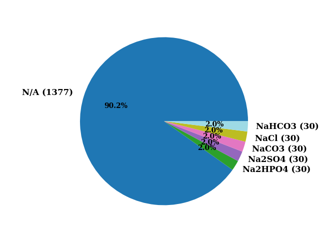
Anions are representative of inorganic content in the xyz.
print(len(data['Anions'].unique()))

data['Anions'].unique()
6

array(['N/A', 'NaCl', 'Na2SO4', 'NaCO3', 'NaHCO3', 'Na2HPO4'],
      dtype=object)
colors, _ = map_array_to_cmap(np.arange(len(data['Anions'].unique())), cmap="tab20")
pie(data['Anions'], colors=colors)
([<matplotlib.patches.Wedge object at 0x796857b82210>, <matplotlib.patches.Wedge object at 0x796857b82420>, <matplotlib.patches.Wedge object at 0x796857b82e10>, <matplotlib.patches.Wedge object at 0x796857b83740>, <matplotlib.patches.Wedge object at 0x796857b83f50>, <matplotlib.patches.Wedge object at 0x796857b17080>], [Text(-1.048034323852062, 0.33410186474779097, 'N/A (1377) '), Text(0.9346079169970015, -0.58009313173535, 'Na2HPO4 (30) '), Text(0.9989222380844521, -0.46060217352977106, 'Na2SO4 (30) '), Text(1.0480344313800127, -0.33410152744633453, 'NaCO3 (30) '), Text(1.0811970815092378, -0.20251634733005408, 'NaCl (30) '), Text(1.097905501694757, -0.067849166158355, 'NaHCO3 (30) ')], [Text(-0.5716550857374884, 0.18223738077152232, '90.2%'), Text(0.509786136543819, -0.31641443549200904, '2.0%'), Text(0.544866675318792, -0.2512375491980569, '2.0%'), Text(0.5716551443890977, -0.18223719678890973, '2.0%'), Text(0.5897438626414023, -0.11046346218002949, '2.0%'), Text(0.5988575463789583, -0.03700863608637545, '2.0%')])
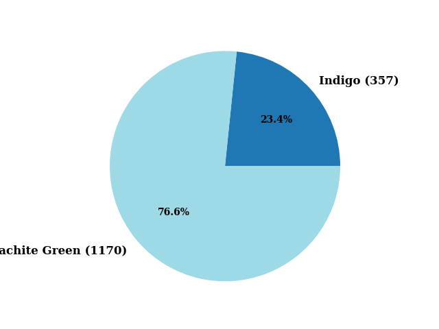
print(len(data['Dye'].unique()))

data['Dye'].unique()
2

array(['Indigo', 'Melachite Green'], dtype=object)
colors, _ = map_array_to_cmap(np.arange(len(data['Dye'].unique())), cmap="tab20")
pie(data['Dye'], colors=colors)
([<matplotlib.patches.Wedge object at 0x7968559323c0>, <matplotlib.patches.Wedge object at 0x796857bf92b0>], [Text(0.8163984327169364, 0.737220183566165, 'Indigo (357) '), Text(-0.8163984672287029, -0.7372201453477955, 'Melachite Green (1170) ')], [Text(0.44530823602741976, 0.4021201001269991, '23.4%'), Text(-0.4453082548520197, -0.40212007928061566, '76.6%')])
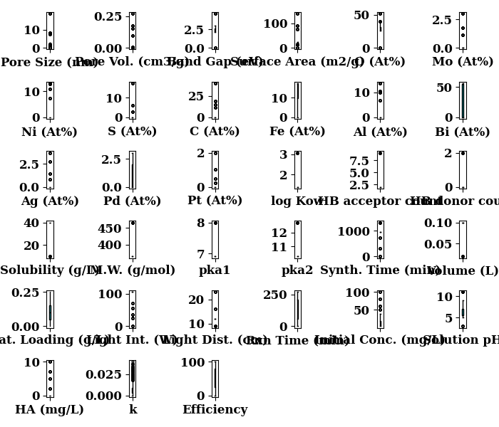
Overall distribution of all features
data_num = data.drop(columns=['Catalyst', 'Anions', 'Dye'])

# rearrange_columns in data_num so that same categories lie close to each other

data_num_ = pd.DataFrame()
for cat, val in CATEGORIES.items():
    for v in val:
        if v in data_num:
            data_num_[v] = data_num[v]
data_num_['k'] = data_num['k']
data_num_['Efficiency'] = data_num['Efficiency']
data_num = data_num_

boxplot(data_num,
        labels=[LABEL_MAP.get(label, label) for label in data_num.columns],
        share_axes=False,
        flierprops=dict(ms=2.0),
        medianprops={"color": "black"},
        fill_color='#01B0B9',
        patch_artist=True,
        show=False,
        figsize=(7, 6),
        )
plt.subplots_adjust(wspace=0.05)
plt.tight_layout()
plt.show()
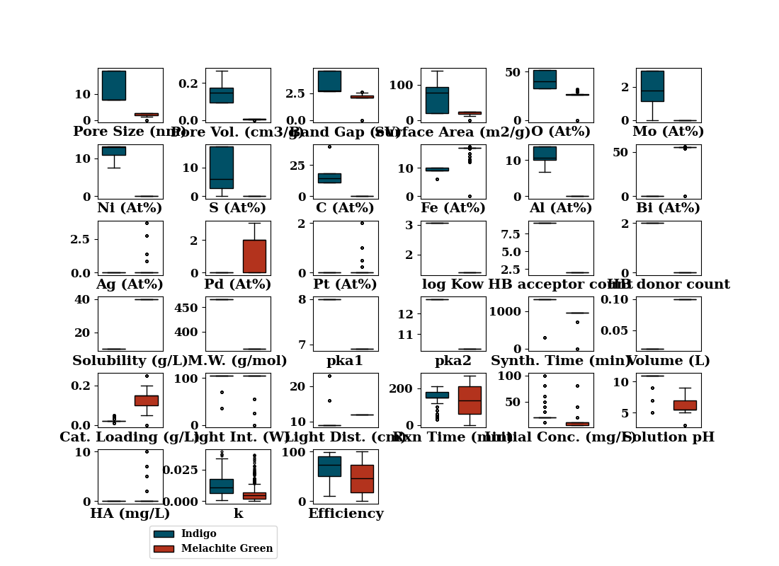
Distribution of a feautre given a specific dye i.e. Dist(Feature)|Dye
grps = data.groupby(by="Dye")

f, axes = create_subplots(data_num.shape[1], figsize=(11, 8))

for col, ax in zip(data_num.columns, axes.flat):

    _, out = boxplot(
    [grps.get_group('Indigo')[col].values, grps.get_group('Melachite Green')[col].values],
        flierprops=dict(ms=2.0),
        medianprops={"color": "black"},
        fill_color=['#005066', '#B3331D'],
        widths=0.7,
        patch_artist=True,
        ax=ax,
        show=False
    )
    ax.set_xlabel(LABEL_MAP.get(col, col))
    ax.set_xticks([])
ax.legend([out["boxes"][0], out["boxes"][1]], ['Indigo', 'Melachite Green'],
          loc=(-2.5, -1))
plt.subplots_adjust(wspace=0.65, hspace=0.4)
if SAVE:
    plt.savefig("results/figures/boxplots.png", dpi=600, bbox_inches="tight")
plt.tight_layout()
plt.show()
/home/docs/checkouts/readthedocs.org/user_builds/weil101/checkouts/latest/scripts/eda.py:146: UserWarning: Tight layout not applied. tight_layout cannot make Axes width small enough to accommodate all Axes decorations
  plt.tight_layout()
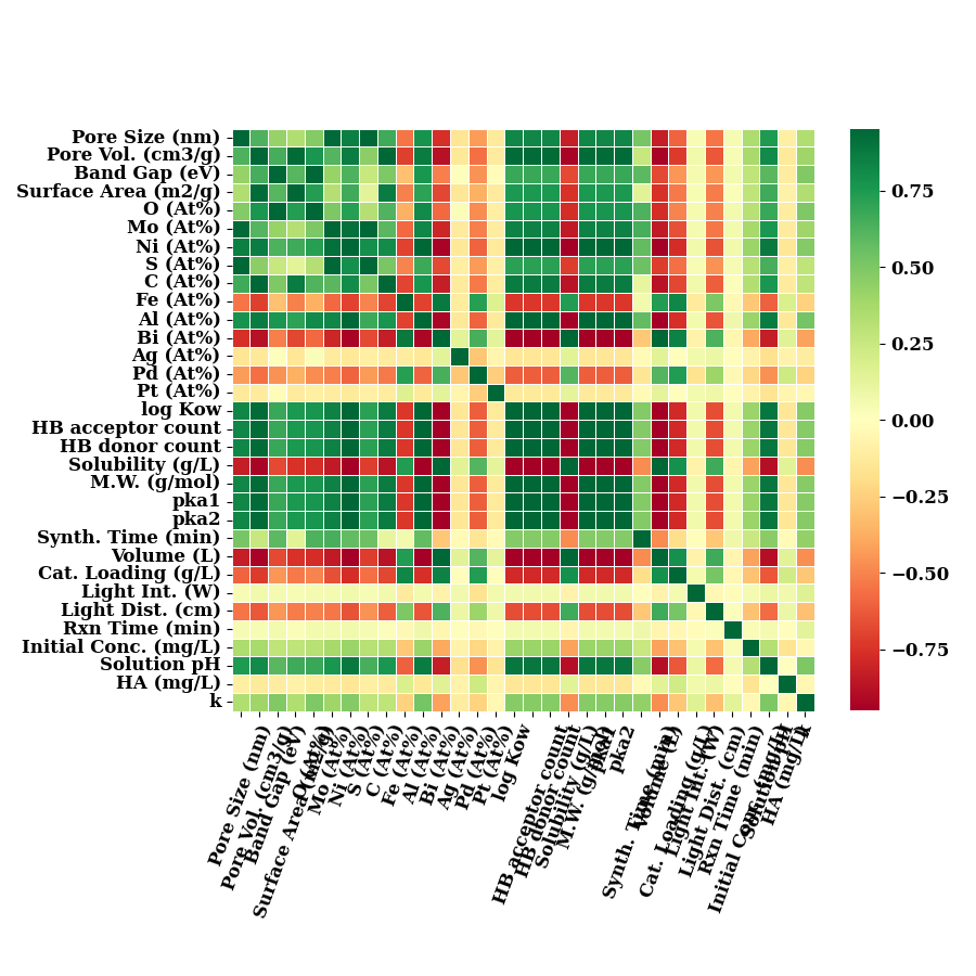
correlation of all input features with k
data_num1 = data_num.rename(columns=LABEL_MAP)
data_num1.pop('Efficiency')
plot_correlation(data_num1, show=False)
if SAVE:
    plt.savefig("results/figures/corr_all_k.png", dpi=600, bbox_inches="tight")
plt.tight_layout()
plt.show()
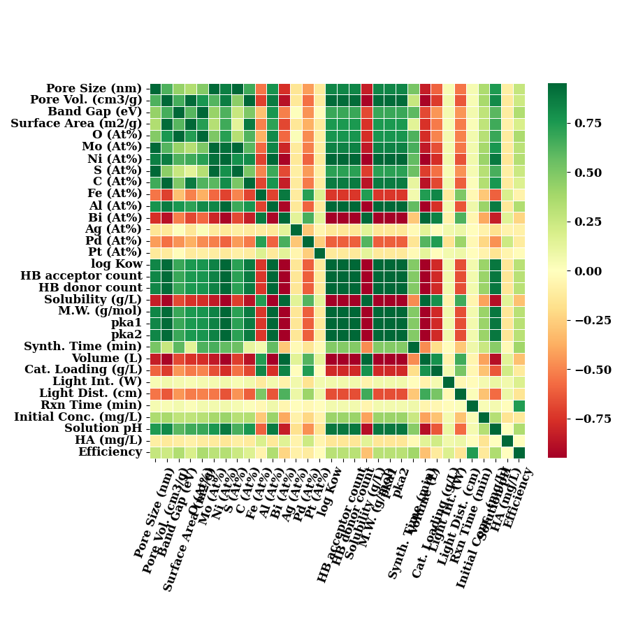
correlation of all input features with Efficiency
data_num1 = data_num.rename(columns=LABEL_MAP)
data_num1.pop('k')
plot_correlation(data_num1)
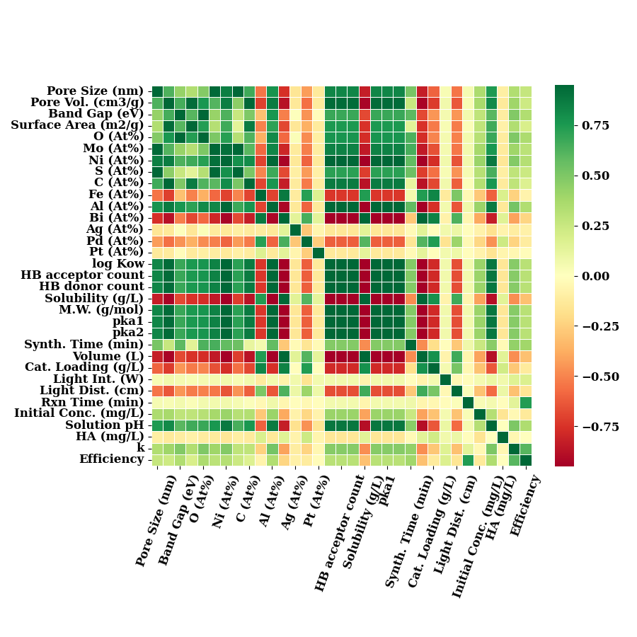
correlation of all input features with Efficiency and k
data_num1 = data_num.rename(columns=LABEL_MAP)

plot_correlation(data_num1, show=False)
if SAVE:
    plt.savefig("results/figures/corr_all_k_e.png", dpi=600, bbox_inches="tight")
plt.tight_layout()
plt.show()
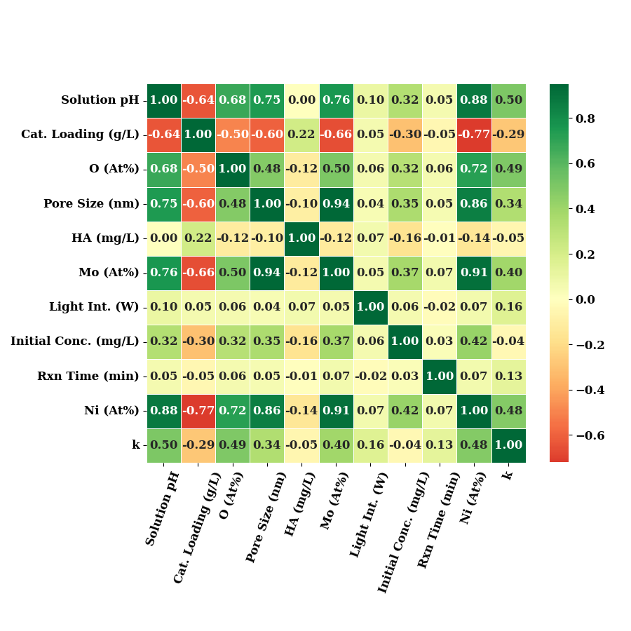
correlation of only input features which were termed as important by Boruta method for k.
cols = ['Solution pH', 'Cat. Loading (g/L)', 'O (At%)', 'Pore Size (nm)',
        'HA (mg/L)', 'Mo (At%)', 'Light Int. (W)', #'Anions',
        'Initial Conc. (mg/L)', 'Rxn Time (min)', 'Ni (At%)']

data_num1 = data_num.rename(columns=LABEL_MAP)[cols + ["k"]]
plot_correlation(data_num1, annot_kws={"fontsize": 12}, show=False)
if SAVE:
    plt.savefig("results/figures/corr_k.png", dpi=600, bbox_inches="tight")
plt.tight_layout()
plt.show()
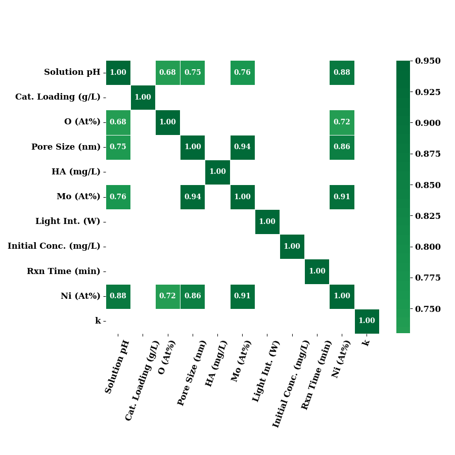
plotting only those where correlation is higher than 0.6
plot_correlation(data_num1, threshold=0.6, split="pos")
plotting only those where correlation is below 0.5
plot_correlation(data_num1, threshold=-0.5, split="neg")

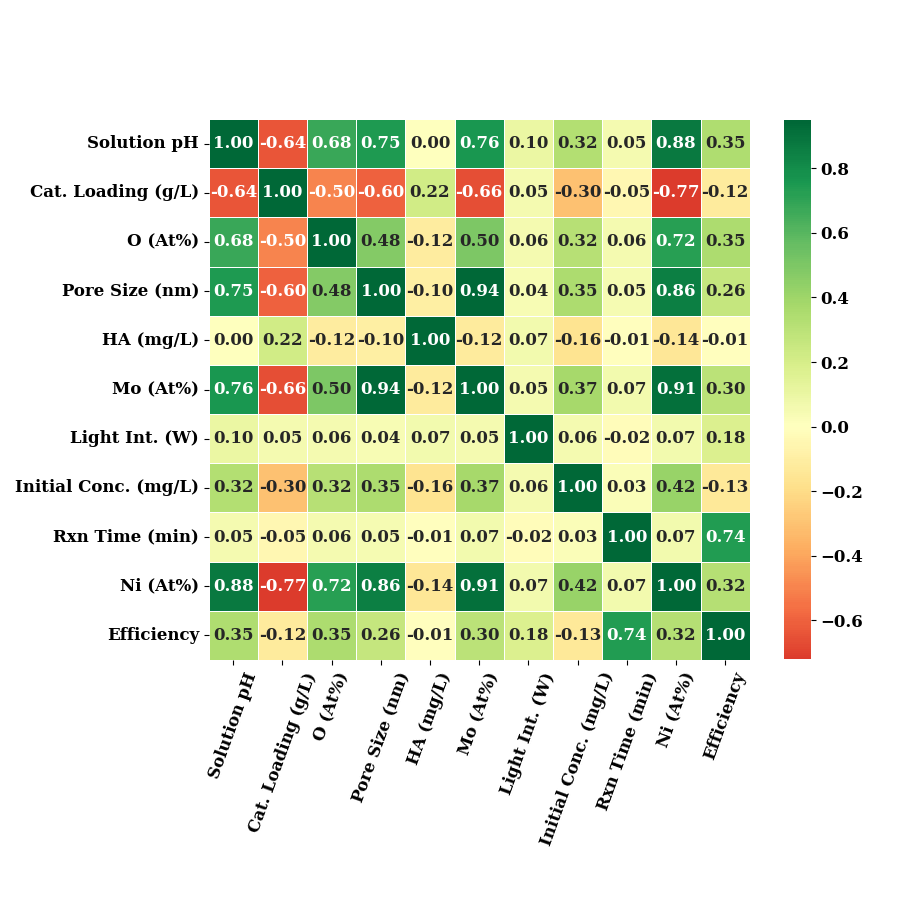
correlation of input features which were termed as important by Boruta method.
data_num1 = data_num.rename(columns=LABEL_MAP)[cols + ["Efficiency"]]
plot_correlation(data_num1, annot_kws={"fontsize": 12})
data_num1 = data_num.rename(columns=LABEL_MAP)[cols + ["k", "Efficiency"]]
plot_correlation(data_num1, annot_kws={"fontsize": 12},
                 show=False)
if SAVE:
    plt.savefig("results/figures/corr_selected.png", dpi=600, bbox_inches="tight")
plt.tight_layout()
plt.show()

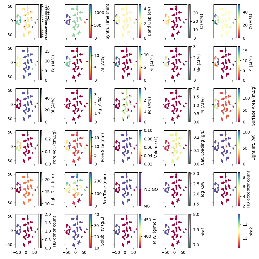
mpl.rcParams.update(mpl.rcParamsDefault)

data, encoders = prepare_data(outputs=["k", "Efficiency"])
input_features = data.columns.tolist()

tsne = TSNE(random_state=313)
comp = tsne.fit_transform(data[input_features])

def scatter_(first, second, label,
             axs, fig):

    c = data[col].values

    pc = axs.scatter(first, second,
                    c=c,
                    s = 2,
            cmap="Spectral",
            )

    if label in ["Catalyst", "Anions", "Dye"]:
        cmap = mpl.cm.Spectral
        bounds = list(set(c))
        norm = mpl.colors.BoundaryNorm(bounds + [bounds[-1]+1],
                                       cmap.N)

        colorbar = fig.colorbar(
            mpl.cm.ScalarMappable(norm=norm, cmap=cmap),
            ticks = bounds,
                 ax=axs, orientation='vertical')

        if label == "Catalyst":
            ticklabels = range(18)
        elif label == "Anions":
            ticklabels = ['N/A', 'Cl', 'SO4', 'CO3', 'HCO3', 'HPO4']
        elif label == "Dye":
            ticklabels = ["MG", "INDIGO"]
        else:
            ticklabels = encoders[label].classes_
        colorbar.ax.set_yticklabels(ticklabels)

    else:
        colorbar = fig.colorbar(pc, ax=axs)
        label = LABEL_MAP.get(label, label)
        colorbar.set_label(label)

    despine_axes(colorbar.ax)
    return
f, axes = create_subplots(29, sharex="all", sharey="all",
                       figsize=(9, 9))

for col, ax in zip(input_features, axes.flat):

    scatter_(comp[:, 0], comp[:, 1],
         label=col, axs=ax, fig=f)

plt.tight_layout()
plt.show()
Total running time of the script: (0 minutes 26.414 seconds)