Note
Go to the end to download the full example code.
3. Feature Selection
Now we know that which model works best for our problem. Now we will perform feature selection using the best model.
import numpy as np

np.NaN = np.nan  # for compatibility with older versions of NumPy
#np.bool = np.bool_  # for compatibility with older versions of NumPy

import seaborn as sns

import matplotlib.pyplot as plt

from easy_mpl import bar_chart

#####  Monkey-patch SciPy before importing BorutaShap because binom_test was renamed to binomtest in SciPy 1.7.0, and BorutaShap uses the old name.
import scipy.stats as stats

# Add the old name if SciPy only has the new one
if not hasattr(stats, "binom_test") and hasattr(stats, "binomtest"):
    def binom_test(x, n=None, p=0.5, alternative="two-sided"):
        return stats.binomtest(int(x), n=n, p=p, alternative=alternative).pvalue
    stats.binom_test = binom_test

#####
from BorutaShap import BorutaShap

from sklearn.tree import DecisionTreeRegressor
from sklearn.feature_selection import RFE
from sklearn.feature_selection import SelectKBest
from sklearn.feature_selection import f_regression
from sklearn.feature_selection import SelectFromModel
from sklearn.feature_selection import VarianceThreshold
from sklearn.feature_selection import mutual_info_regression
from sklearn.feature_selection import SequentialFeatureSelector

from utils import set_rcParams
from utils import version_info
from utils import prepare_data, LABEL_MAP, SAVE
for lib, ver in version_info().items():
    print(lib, ver)
python 3.12.10 (main, May  6 2025, 10:49:23) [GCC 11.4.0]
os posix
ai4water 1.07
lightgbm 4.6.0
catboost 1.2.10
xgboost 3.2.0
easy_mpl 0.21.5
SeqMetrics 2.0.0
numpy 1.26.4
pandas 2.2.3
matplotlib 3.10.8
h5py 3.16.0
sklearn 1.3.1
optuna 4.8.0
skopt 0.10.2
plotly 6.6.0
seaborn 0.13.2
crepes 0.9.0
mapie 0.9.2
shap 0.49.1
scipy 1.17.1
set_rcParams()

TOP_K = 10

df, _ = prepare_data(outputs="k")

df = df.rename(columns=LABEL_MAP)

feature_names = df.columns.tolist()[0:-1]

X, y = df.iloc[:, 0:-1], df.iloc[:, -1].values

print(X.shape, y.shape)
(1527, 34) (1527,)
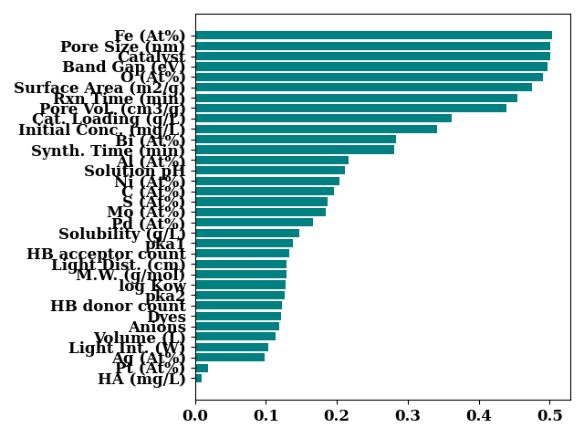
Information gain
importances = mutual_info_regression(
    X, y)

bar_chart(
    importances,
    feature_names,
    color="teal",
    sort=True,
    show=False,
)
plt.tight_layout()
plt.show()
Chi-squared
chi2_features = SelectKBest(f_regression, k=10)
X_kbest_features = chi2_features.fit_transform(
    X, y)

chi2_features = np.array(feature_names)[chi2_features.get_support()]
print(chi2_features)

chi2_features = chi2_features[0:TOP_K].tolist()
['Band Gap (eV)' 'O (At%)' 'Al (At%)' 'Ni (At%)' 'Volume (L)'
 'HB donor count' 'Solubility (g/L)' 'M.W. (g/mol)' 'pka2' 'Solution pH']
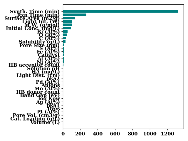
Variance Threshold
v_threshold = VarianceThreshold(threshold=0)
v_threshold.fit(X)
v_threshold.get_support()

bar_chart(
    v_threshold.variances_,
    feature_names,
    color="teal",
    sort=True,
    show=False
)
plt.tight_layout()
plt.show()

vt_features = {k:v for k,v in zip(v_threshold.variances_, feature_names, )}
# sort_by_value
vt_features =  dict(sorted(vt_features.items(), key=lambda item: item[1], reverse=True))
vt_features = np.array(list(vt_features.values()))[0:TOP_K].tolist()
Forward Feature Selection
Starting with empty/minimal feature set and adding features one by one
rgr = DecisionTreeRegressor()
sfs_forward = SequentialFeatureSelector(
    rgr, n_features_to_select=TOP_K, direction="forward"
).fit(X, y)

ffs_features = np.array(feature_names)[sfs_forward.get_support()]
print(ffs_features)

ffs_features = ffs_features.tolist()
['Al (At%)' 'Ni (At%)' 'Pt (At%)' 'Light Int. (W)' 'Light Dist. (cm)'
 'HB acceptor count' 'pka2' 'Initial Conc. (mg/L)' 'Solution pH'
 'HA (mg/L)']
Backward feature elimination
Starting with a full set of features and removing one by one and everytime measuring the decrease in performance. Finally we rank the features, according to the decrease in performance they cause.
sfs_forward = SequentialFeatureSelector(
    rgr, n_features_to_select=TOP_K, direction="backward"
).fit(X, y)

bfe_features = np.array(feature_names)[sfs_forward.get_support()]
print(bfe_features)

bfe_features = bfe_features.tolist()
['Catalyst' 'Al (At%)' 'Pt (At%)' 'Surface Area (m2/g)' 'Light Dist. (cm)'
 'Rxn Time (min)' 'Dyes' 'log Kow' 'HB donor count' 'Initial Conc. (mg/L)']
Recursive Feeature Elimination
It is similar to backward feature elemination.
rfe = RFE(DecisionTreeRegressor(), n_features_to_select=TOP_K,
          step=1)
rfe.fit(X, y)
rfe_features = np.array(feature_names)[rfe.get_support()]
print(rfe_features)

rfe_features = rfe_features[0:TOP_K].tolist()
['O (At%)' 'Al (At%)' 'Pore Vol. (cm3/g)' 'Cat. Loading (g/L)'
 'Light Int. (W)' 'Rxn Time (min)' 'Initial Conc. (mg/L)' 'Solution pH'
 'HA (mg/L)' 'Anions']
Tree based method
rgr = DecisionTreeRegressor().fit(X, y)
model = SelectFromModel(rgr, prefit=True)

tb_features = np.array(feature_names)[model.get_support()]
print(tb_features)

tb_features = tb_features[0:TOP_K].tolist()
['Al (At%)' 'Ni (At%)' 'Cat. Loading (g/L)' 'Light Int. (W)'
 'Rxn Time (min)' 'Initial Conc. (mg/L)' 'Solution pH' 'Anions']
Boruta shap
The purpose of Boruta is to find a subset of features from all the given features, which are relevant for the given task. It creats a copy of a feature which is called shadow feature. Then the shadow feature is shuffled. The model is trained with the original feature plus the shuffled shadow feature. After that the feature importance of the original feature and shadow feature is calcualted using SHAP. If the SHAP importance of a shadow feature is more than the orignal feature, then it is rejected. The intuition is that, if a feature is important, then its shuffled version should not have more importnace than the original feature. Finally, Boruta shap method groups features, either as confirmed important, or confirmed rejected or tentative features. Since Boruta involves training the original model again and again, this can be extremely costly if the model training is time consuming. For theory see this article and this kaggle notebook .
class MyBoruta(BorutaShap):
    def box_plot(self, data, X_rotation, X_size, y_scale, figsize):

        if y_scale=='log':
            minimum = data['value'].min()
            if minimum <= 0:
                data['value'] += abs(minimum) + 0.01

        order = data.groupby(by=["Methods"])["value"].mean().sort_values(ascending=False).index
        my_palette = self.create_mapping_of_features_to_attribute(
            maps= ['#B17BB2', '#EE9E9D', '#00ABAC',  '#B9E6FB'])
                 # 'yellow',   'red',     'green',    'blue'

        # Use a color palette
        plt.figure(figsize=(10, 7))
        ax = sns.boxplot(x=data["Methods"], y=data["value"],
                        order=order, palette=my_palette)

        if y_scale == 'log':ax.set(yscale="log")
        ax.set_xticklabels(ax.get_xticklabels(), rotation=X_rotation, size=14)
        ax.tick_params(labelsize=14)
        ax.grid(visible=True, ls='--', color='lightgrey')
        ax.set_ylabel('Z-Score', fontsize=14)
        ax.set_xlabel('Features', fontsize=14,)
        plt.tight_layout()

        if SAVE:
            plt.savefig("results/figures/boruta_shap.png", dpi=600, bbox_inches="tight")
        return
model = DecisionTreeRegressor()
Feature_Selector = MyBoruta(model=model,
                              importance_measure='shap',
                              classification=False)
We observed that the number of confirmed important and tentative
features remained same after 50 n_trials. At 50 n_trials
the total potential features were 12. Further increasing
the n_trials only moved the features from ‘tentative’ category
to ‘confirmed important’ until 400. For computational constraints on
readthedocs, we are setting n_trials to 100.
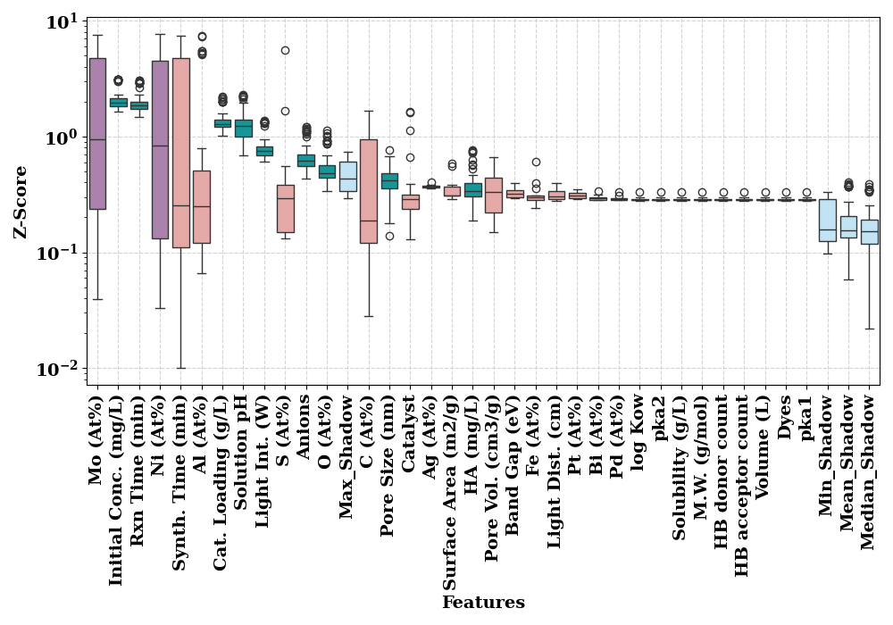
z_score on y-axis is a measure of importance and therefore, boxplots
display the distribution of importance.
Feature_Selector.fit(
    X=X, y=y,
     n_trials=100,
     sample=False,
     train_or_test = 'test',
     normalize=True,
    verbose=True
)
  0%|          | 0/100 [00:00<?, ?it/s]
  1%|          | 1/100 [00:00<01:08,  1.45it/s]
  2%|▏         | 2/100 [00:01<01:05,  1.50it/s]
  3%|▎         | 3/100 [00:01<01:01,  1.57it/s]
  4%|▍         | 4/100 [00:02<01:02,  1.53it/s]
  5%|▌         | 5/100 [00:03<01:00,  1.57it/s]
  6%|▌         | 6/100 [00:03<01:00,  1.56it/s]
  7%|▋         | 7/100 [00:04<01:00,  1.53it/s]
  8%|▊         | 8/100 [00:05<00:58,  1.57it/s]
  9%|▉         | 9/100 [00:05<00:59,  1.52it/s]
 10%|█         | 10/100 [00:06<00:58,  1.54it/s]
 11%|█         | 11/100 [00:07<00:57,  1.55it/s]
 12%|█▏        | 12/100 [00:07<00:55,  1.59it/s]
 13%|█▎        | 13/100 [00:08<00:55,  1.57it/s]
 14%|█▍        | 14/100 [00:08<00:52,  1.64it/s]
 15%|█▌        | 15/100 [00:09<00:51,  1.66it/s]
 16%|█▌        | 16/100 [00:10<00:49,  1.71it/s]
 17%|█▋        | 17/100 [00:10<00:48,  1.72it/s]
 18%|█▊        | 18/100 [00:11<00:47,  1.73it/s]
 19%|█▉        | 19/100 [00:11<00:44,  1.81it/s]
 20%|██        | 20/100 [00:12<00:44,  1.78it/s]
 21%|██        | 21/100 [00:12<00:45,  1.74it/s]
 22%|██▏       | 22/100 [00:13<00:44,  1.77it/s]
 23%|██▎       | 23/100 [00:13<00:43,  1.77it/s]
 24%|██▍       | 24/100 [00:14<00:42,  1.80it/s]
 25%|██▌       | 25/100 [00:15<00:41,  1.81it/s]
 26%|██▌       | 26/100 [00:15<00:41,  1.78it/s]
 27%|██▋       | 27/100 [00:16<00:42,  1.72it/s]
 28%|██▊       | 28/100 [00:16<00:40,  1.78it/s]
 29%|██▉       | 29/100 [00:17<00:38,  1.85it/s]
 30%|███       | 30/100 [00:17<00:37,  1.87it/s]
 31%|███       | 31/100 [00:18<00:36,  1.91it/s]
 32%|███▏      | 32/100 [00:18<00:35,  1.91it/s]
 33%|███▎      | 33/100 [00:19<00:35,  1.91it/s]
 34%|███▍      | 34/100 [00:19<00:34,  1.89it/s]
 35%|███▌      | 35/100 [00:20<00:33,  1.92it/s]
 36%|███▌      | 36/100 [00:20<00:32,  1.99it/s]
 37%|███▋      | 37/100 [00:21<00:31,  2.01it/s]
 38%|███▊      | 38/100 [00:21<00:31,  1.97it/s]
 39%|███▉      | 39/100 [00:22<00:30,  2.00it/s]
 40%|████      | 40/100 [00:22<00:31,  1.90it/s]
 41%|████      | 41/100 [00:23<00:30,  1.91it/s]
 42%|████▏     | 42/100 [00:23<00:30,  1.93it/s]
 43%|████▎     | 43/100 [00:24<00:28,  1.97it/s]
 44%|████▍     | 44/100 [00:24<00:28,  1.95it/s]
 45%|████▌     | 45/100 [00:25<00:27,  1.98it/s]
 46%|████▌     | 46/100 [00:25<00:27,  1.94it/s]
 47%|████▋     | 47/100 [00:26<00:27,  1.93it/s]
 48%|████▊     | 48/100 [00:27<00:26,  1.96it/s]
 49%|████▉     | 49/100 [00:27<00:25,  1.98it/s]
 50%|█████     | 50/100 [00:28<00:25,  1.98it/s]
 51%|█████     | 51/100 [00:28<00:25,  1.94it/s]
 52%|█████▏    | 52/100 [00:29<00:24,  1.95it/s]
 53%|█████▎    | 53/100 [00:29<00:23,  1.96it/s]
 54%|█████▍    | 54/100 [00:30<00:23,  1.95it/s]
 55%|█████▌    | 55/100 [00:30<00:22,  1.96it/s]
 56%|█████▌    | 56/100 [00:31<00:22,  1.96it/s]
 57%|█████▋    | 57/100 [00:31<00:22,  1.91it/s]
 58%|█████▊    | 58/100 [00:32<00:21,  1.94it/s]
 59%|█████▉    | 59/100 [00:32<00:20,  1.97it/s]
 60%|██████    | 60/100 [00:33<00:20,  1.96it/s]
 61%|██████    | 61/100 [00:33<00:19,  1.97it/s]
 62%|██████▏   | 62/100 [00:34<00:19,  1.90it/s]
 63%|██████▎   | 63/100 [00:34<00:19,  1.92it/s]
 64%|██████▍   | 64/100 [00:35<00:18,  1.92it/s]
 65%|██████▌   | 65/100 [00:35<00:18,  1.88it/s]
 66%|██████▌   | 66/100 [00:36<00:18,  1.87it/s]
 67%|██████▋   | 67/100 [00:36<00:17,  1.93it/s]
 68%|██████▊   | 68/100 [00:37<00:16,  1.94it/s]
 69%|██████▉   | 69/100 [00:37<00:16,  1.91it/s]
 70%|███████   | 70/100 [00:38<00:15,  1.91it/s]
 71%|███████   | 71/100 [00:38<00:14,  1.96it/s]
 72%|███████▏  | 72/100 [00:39<00:14,  1.94it/s]
 73%|███████▎  | 73/100 [00:39<00:13,  1.93it/s]
 74%|███████▍  | 74/100 [00:40<00:13,  1.95it/s]
 75%|███████▌  | 75/100 [00:40<00:13,  1.90it/s]
 76%|███████▌  | 76/100 [00:41<00:12,  1.88it/s]
 77%|███████▋  | 77/100 [00:42<00:12,  1.90it/s]
 78%|███████▊  | 78/100 [00:42<00:11,  1.90it/s]
 79%|███████▉  | 79/100 [00:43<00:11,  1.90it/s]
 80%|████████  | 80/100 [00:43<00:10,  1.89it/s]
 81%|████████  | 81/100 [00:44<00:09,  1.92it/s]
 82%|████████▏ | 82/100 [00:44<00:09,  1.97it/s]
 83%|████████▎ | 83/100 [00:45<00:08,  2.00it/s]
 84%|████████▍ | 84/100 [00:45<00:07,  2.08it/s]
 85%|████████▌ | 85/100 [00:45<00:07,  2.10it/s]
 86%|████████▌ | 86/100 [00:46<00:06,  2.11it/s]
 87%|████████▋ | 87/100 [00:46<00:06,  2.07it/s]
 88%|████████▊ | 88/100 [00:47<00:05,  2.05it/s]
 89%|████████▉ | 89/100 [00:47<00:05,  2.05it/s]
 90%|█████████ | 90/100 [00:48<00:04,  2.12it/s]
 91%|█████████ | 91/100 [00:48<00:04,  2.15it/s]
 92%|█████████▏| 92/100 [00:49<00:03,  2.11it/s]
 93%|█████████▎| 93/100 [00:49<00:03,  2.16it/s]
 94%|█████████▍| 94/100 [00:50<00:02,  2.13it/s]
 95%|█████████▌| 95/100 [00:50<00:02,  2.12it/s]
 96%|█████████▌| 96/100 [00:51<00:01,  2.10it/s]
 97%|█████████▋| 97/100 [00:51<00:01,  2.08it/s]
 98%|█████████▊| 98/100 [00:52<00:00,  2.06it/s]
 99%|█████████▉| 99/100 [00:52<00:00,  2.09it/s]
100%|██████████| 100/100 [00:53<00:00,  2.08it/s]
100%|██████████| 100/100 [00:53<00:00,  1.88it/s]
9 attributes confirmed important: ['HA (mg/L)', 'Anions', 'Rxn Time (min)', 'Light Int. (W)', 'Pore Size (nm)', 'Initial Conc. (mg/L)', 'Solution pH', 'Cat. Loading (g/L)', 'O (At%)']
23 attributes confirmed unimportant: ['M.W. (g/mol)', 'Dyes', 'Catalyst', 'Synth. Time (min)', 'Pt (At%)', 'Solubility (g/L)', 'Band Gap (eV)', 'C (At%)', 'Volume (L)', 'Pd (At%)', 'HB acceptor count', 'Al (At%)', 'HB donor count', 'Fe (At%)', 'Surface Area (m2/g)', 'log Kow', 'pka2', 'S (At%)', 'Light Dist. (cm)', 'Pore Vol. (cm3/g)', 'Bi (At%)', 'pka1', 'Ag (At%)']
2 tentative attributes remains: ['Ni (At%)', 'Mo (At%)']
Boxplot of features. Features with grass green color are considered as confirmed important. The orange color represents confirmed rejected/unimportant.
Feature_Selector.plot()
if SAVE:
    Feature_Selector.results_to_csv('results/Boruta_results.csv')
get the names selected features
print(Feature_Selector.Subset().columns)

br_features = Feature_Selector.Subset().columns[0:TOP_K].tolist()
Index(['HA (mg/L)', 'Anions', 'Rxn Time (min)', 'Light Int. (W)',
       'Pore Size (nm)', 'Initial Conc. (mg/L)', 'Solution pH',
       'Cat. Loading (g/L)', 'O (At%)'],
      dtype='object')
printing the common features among all methods
mi_features = {k:v for k,v in zip(feature_names, importances)}
# sort_by_value
mi_features =  dict(sorted(mi_features.items(), key=lambda item: item[1], reverse=True))
mi_features = np.array(list(mi_features.keys()))[0:TOP_K].tolist()

print(set(
    br_features + mi_features + chi2_features + vt_features +\
    ffs_features + bfe_features + rfe_features
))
{'Dyes', 'Catalyst', 'Synth. Time (min)', 'Light Int. (W)', 'Pt (At%)', 'Pore Size (nm)', 'Solubility (g/L)', 'Initial Conc. (mg/L)', 'Solution pH', 'Band Gap (eV)', 'Volume (L)', 'HB acceptor count', 'Ni (At%)', 'pka1', 'Al (At%)', 'HB donor count', 'O (At%)', 'Fe (At%)', 'Surface Area (m2/g)', 'log Kow', 'pka2', 'Anions', 'S (At%)', 'Cat. Loading (g/L)', 'Light Dist. (cm)', 'HA (mg/L)', 'Pore Vol. (cm3/g)', 'Rxn Time (min)', 'M.W. (g/mol)'}
Total running time of the script: (1 minutes 4.752 seconds)