Note
Go to the end to download the full example code.
6. Interpretation
The purpose of this notebook is to apply various post-hoc interpretation methods on our model. For this purose, we will rebuild our DecisionTree model, train it. After this we will apply SHAP, PDP and ALE on the trained DecisionTree model.
import numpy as np
import pandas as pd

#np.bool = np.bool_

import shap

import matplotlib as mpl
import matplotlib.pyplot as plt

import matplotlib.colors as mcolors

from easy_mpl import pie
from easy_mpl import bar_chart
from easy_mpl.utils import create_subplots

from shap.plots import waterfall
from shap import summary_plot, Explanation

from ai4water import Model
from ai4water.utils.utils import TrainTestSplit
from ai4water.postprocessing import PartialDependencePlot

from utils import LABEL_MAP
from utils import version_info
from utils import shap_scatter
from utils import make_classes
from utils import shap_scatter_plots
from utils import prepare_data, set_rcParams, plot_ale, SAVE
for lib, ver in version_info().items():
    print(lib, ver)
python 3.12.10 (main, May  6 2025, 10:49:23) [GCC 11.4.0]
os posix
ai4water 1.07
lightgbm 4.6.0
catboost 1.2.10
xgboost 3.2.0
easy_mpl 0.21.5
SeqMetrics 2.0.0
numpy 1.26.4
pandas 2.2.3
matplotlib 3.10.8
h5py 3.16.0
sklearn 1.3.1
optuna 4.8.0
skopt 0.10.2
plotly 6.6.0
seaborn 0.13.2
crepes 0.9.0
mapie 0.9.2
shap 0.49.1
scipy 1.17.1
set_rcParams()
inputs = ['Solution pH', 'Time (m)', 'Anions', 'Ni (At%)', 'HA (mg/L)',
          'loading (g)', 'Pore size (nm)', 'O (At%)',
          'Light intensity (watt)', 'Mo (At%)', 'Dye concentration (mg/L)']
data, encoders = prepare_data(inputs=inputs,
                              outputs="k")

print(data.shape)
(1527, 12)
input_features = data.columns.tolist()[0:-1]
output_features = data.columns.tolist()[-1:]

TrainX, TestX, TrainY, TestY = TrainTestSplit(seed=313).split_by_random(
    data[input_features],
    data[output_features]
)

print(TrainX.shape, TrainY.shape, TestX.shape, TestY.shape)

model = Model(
    model = "DecisionTreeRegressor",
    input_features=input_features,
    output_features=output_features,
    verbosity=-1,
)

model.fit(TrainX, TrainY.values)
(1068, 11) (1068, 1) (459, 11) (459, 1)
train_p = model.predict(TrainX, process_results=False)
test_p = model.predict(TestX, process_results=False)
Average prediction on training data
print(train_p.mean())
0.006940225438833623
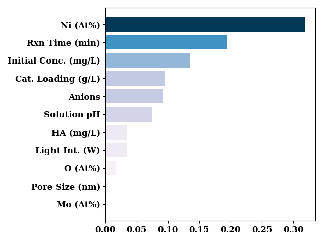
default feature importance from decision tree
print(model._model.feature_importances_)
[7.40882935e-02 1.94588607e-01 9.18145954e-02 3.19367156e-01
 3.43836446e-02 9.41130328e-02 5.70019588e-03 1.71579275e-02
 3.37566239e-02 2.51049444e-04 1.34778874e-01]
bar_chart(model._model.feature_importances_,
          [LABEL_MAP[n] if n in LABEL_MAP else n for n in model.input_features],
          sort=True,
          show=False)
plt.tight_layout()
plt.show()
SHAP
exp = shap.TreeExplainer(model=model._model,
                         data=TrainX,
                         feature_names=input_features)

print(exp.expected_value)
0.0066904566801259955
shap_values = exp.shap_values(TrainX, TrainY)

summary_plot(shap_values,
    TrainX,
    max_display=34,
    feature_names=[LABEL_MAP[n] if n in LABEL_MAP else n for n in input_features],
    show=False)
if SAVE:
    plt.savefig("results/figures/shap_summary.png", dpi=600, bbox_inches="tight")
plt.tight_layout()
plt.show()

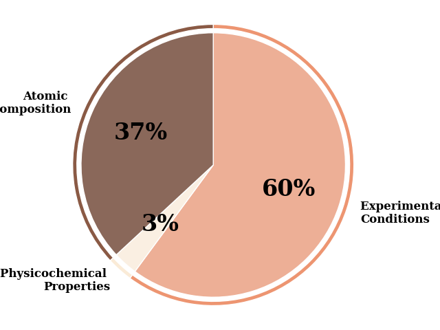
sv_bar = np.mean(np.abs(shap_values), axis=0)

classes, colors, colors_ = make_classes(exp)

df_with_classes = pd.DataFrame({'features': exp.feature_names,
                   'classes': classes,
                   'mean_shap': sv_bar})

print(df_with_classes)
                    features                     classes  mean_shap
0                Solution pH     Experimental Conditions   0.001051
1                   Time (m)     Experimental Conditions   0.001239
2                     Anions     Experimental Conditions   0.000390
3                   Ni (At%)          Atomic Composition   0.003584
4                  HA (mg/L)     Experimental Conditions   0.000281
5                loading (g)     Experimental Conditions   0.001199
6             Pore size (nm)  Physicochemical Properties   0.000322
7                    O (At%)          Atomic Composition   0.000349
8     Light intensity (watt)     Experimental Conditions   0.000395
9                   Mo (At%)          Atomic Composition   0.000014
10  Dye concentration (mg/L)     Experimental Conditions   0.001875
f, ax = plt.subplots(figsize=(7,9))
ax = bar_chart(
    sv_bar,
    [LABEL_MAP[n] if n in LABEL_MAP else n for n in exp.feature_names],
    bar_labels=np.round(sv_bar, 4),
    bar_label_kws={'label_type':'edge',
                   'fontsize': 10,
                   'weight': 'bold',
                   "fmt": '%.4f',
                   'padding': 1.5
                   },
    show=False,
    sort=True,
    color=colors_,
    ax = ax
)
ax.spines[['top', 'right']].set_visible(False)
ax.set_xlabel(xlabel='mean(|SHAP value|)')
ax.set_xticklabels(ax.get_xticks().astype(float))
ax.set_yticklabels(ax.get_yticklabels())

labels = df_with_classes['classes'].unique()
handles = [plt.Rectangle((0,0),1,1,
                         color=colors[l]) for l in labels]
plt.legend(handles, labels, loc='lower right')
ax.xaxis.set_major_locator(plt.MaxNLocator(4))
if SAVE:
    plt.savefig("results/figures/shap_bar.png", dpi=600, bbox_inches="tight")
plt.tight_layout()
plt.show()

seg_colors = (colors.values())
# Change the saturation of seg_colors to 70% for the interior segments
rgb = mcolors.to_rgba_array(seg_colors)[:,:-1]
hsv = mcolors.rgb_to_hsv(rgb)
hsv[:,1] = 0.7 * hsv[:, 1]
interior_colors = mcolors.hsv_to_rgb(hsv)

fractions = np.array([
df_with_classes.loc[df_with_classes['classes']=='Experimental Conditions']['mean_shap'].sum(),
df_with_classes.loc[df_with_classes['classes']=='Physicochemical Properties']['mean_shap'].sum(),
df_with_classes.loc[df_with_classes['classes']=='Atomic Composition']['mean_shap'].sum(),
])

dye_frac = df_with_classes.loc[df_with_classes['classes']=='Dye Properties']['mean_shap'].sum()
labels = ['Experimental \nConditions', 'Physicochemical \nProperties',
               'Atomic \nComposition']

if dye_frac > 0.0:
    fractions = np.array(fractions.tolist().append(dye_frac))
    labels.append('Dye Properties')

fractions /=fractions.sum()

_, texts= pie(fractions=fractions,
    colors=seg_colors,
    labels=labels,
    wedgeprops=dict(edgecolor="w", width=0.03), radius=1,
    autopct=None,
    textprops = dict(fontsize=12),
    startangle=90, counterclock=False, show=False)
texts[0].set_fontsize(12)
_, texts, autotexts = pie(fractions=fractions,
    colors=interior_colors,
       autopct='%1.0f%%',
    textprops = dict(fontsize=24),
    wedgeprops=dict(edgecolor="w"), radius=1-2*0.03,
    startangle=90, counterclock=False, ax=plt.gca(), show=False)
texts[0].set_fontsize(12)
if SAVE:
    plt.savefig("results/figures/shap_pie.png", dpi=600, bbox_inches="tight")
plt.tight_layout()
plt.show()
index = train_p.argmax()
print(index, train_p.max())
355 0.036809739452414975
e = Explanation(
    shap_values[index],
    base_values=exp.expected_value,
    data=TrainX.values[index],
    feature_names=input_features
)

waterfall(e, max_display=20, show=False)
if SAVE:
    plt.savefig(f"results/figures/shap_local_{index}.png", dpi=600, bbox_inches="tight")
plt.tight_layout()
plt.show()

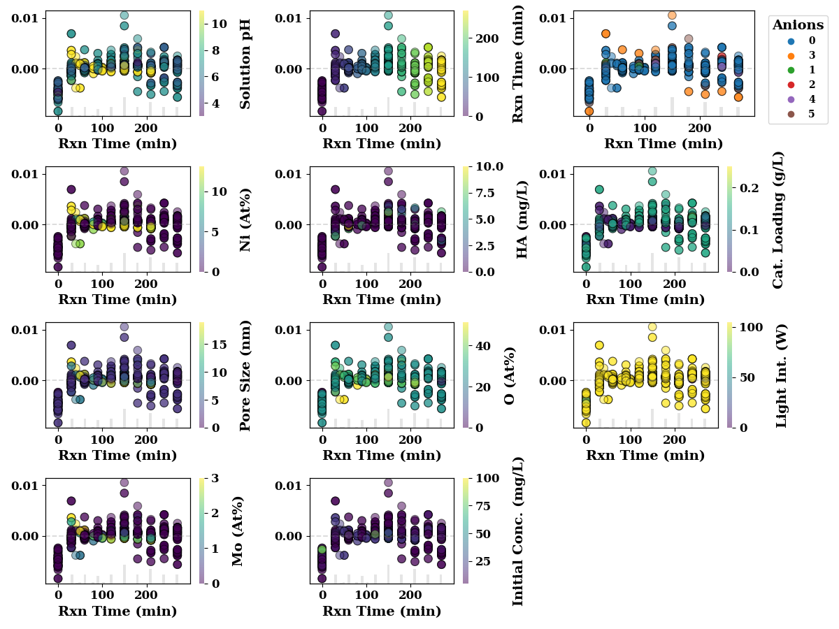
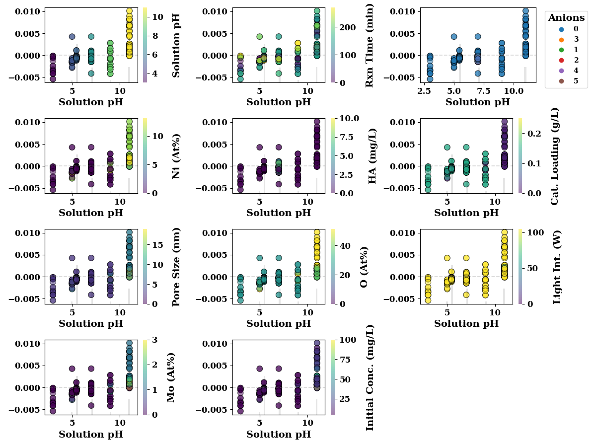
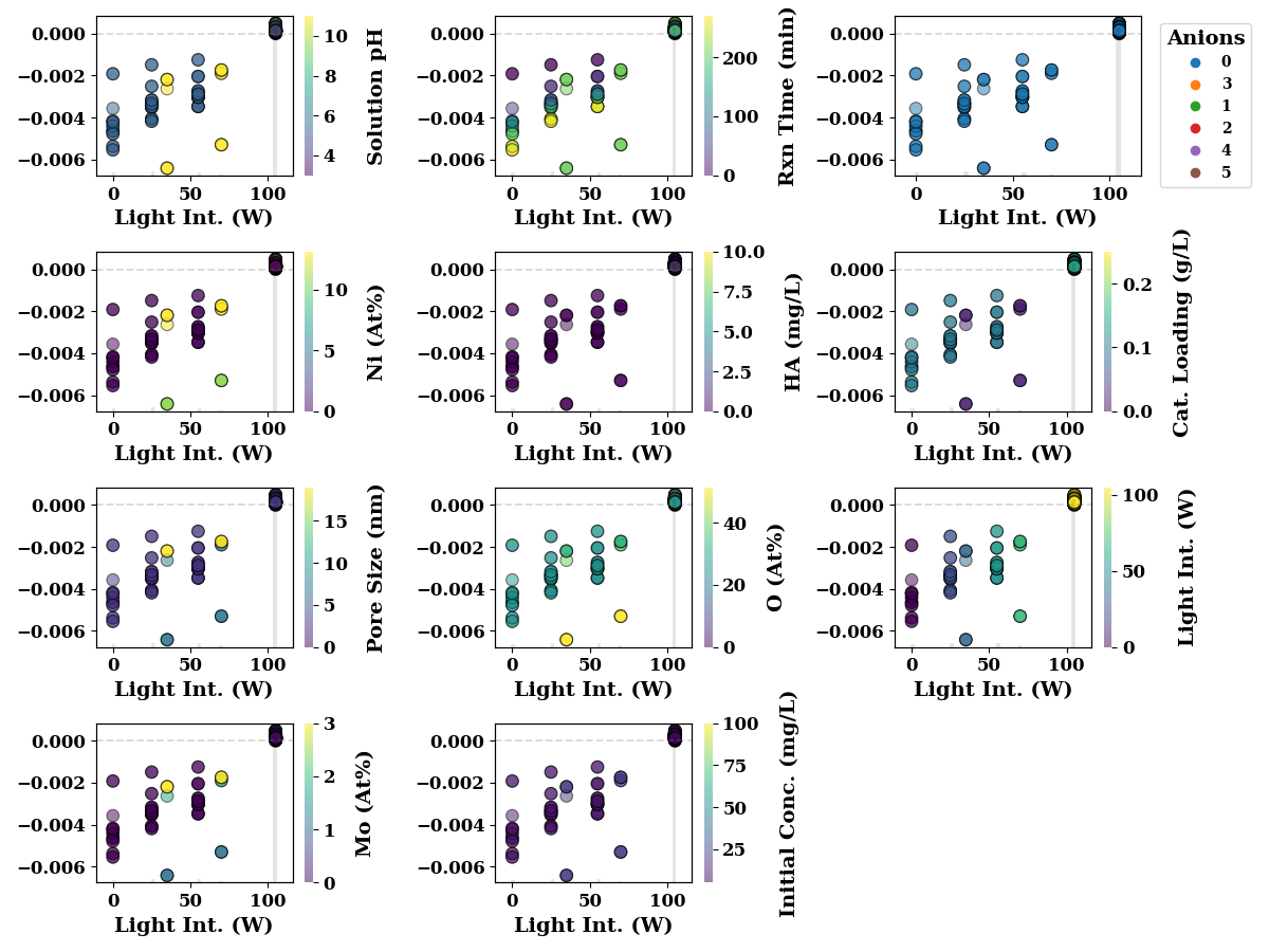
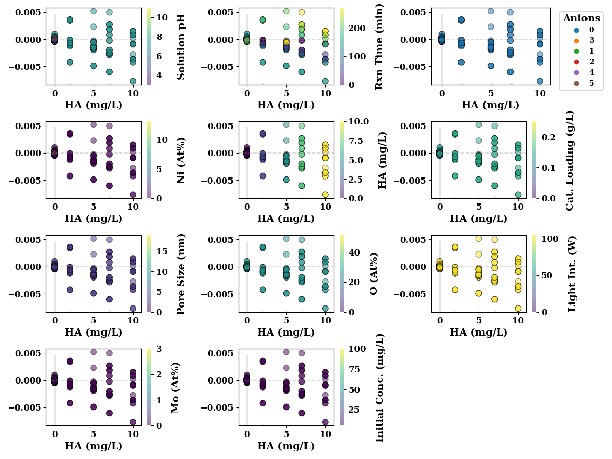
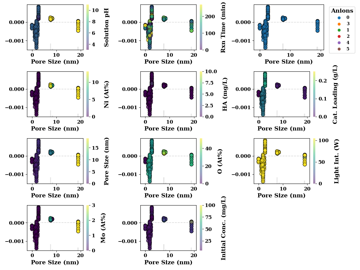
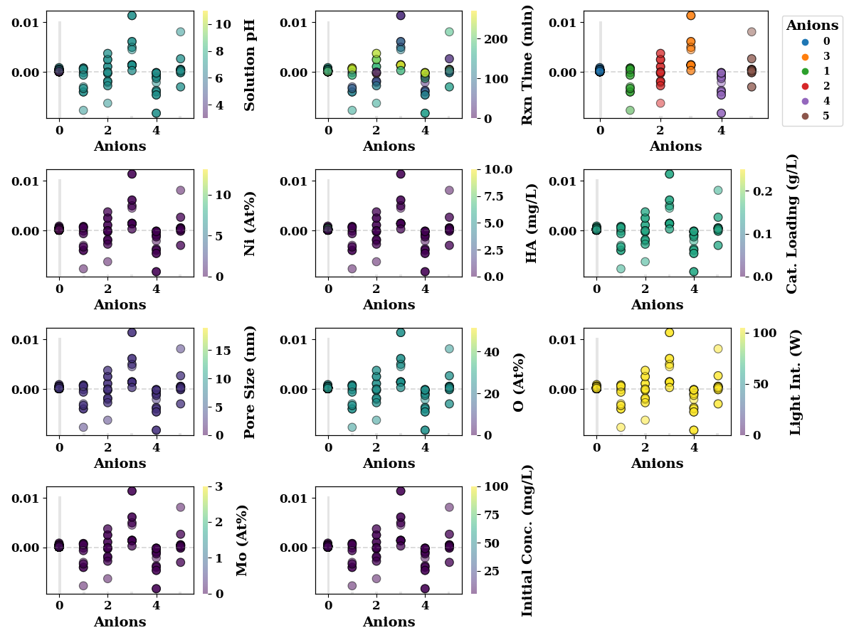
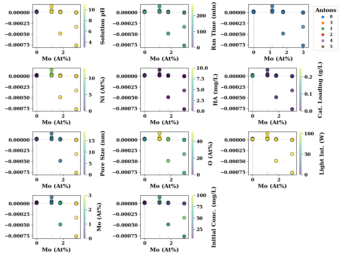
The following figures show SHAP interaction plots. These figures depict the inteaction effect of two features on model performance. In these figures, the numbers in legends for Anions, have following meanings
encoders['Anions'].inverse_transform(np.array([0,1,2,3,4, 5, 5]).reshape(-1,1))
array(['N/A', 'Na2HPO4', 'Na2SO4', 'NaCO3', 'NaCl', 'NaHCO3', 'NaHCO3'],
      dtype=object)
Similarly for catalyst, the numbers in legend have following meanings Pt-BFO : 6 Pd-BFO: 4 LM : 2 Ag-BFO : 0 Photolysis : 5 LTH : 3 BFO : 1
Dye Concentration
It represents initial concentration of dye.
feature_name = 'Dye concentration (mg/L)'

if feature_name in TrainX:
    shap_scatter_plots(shap_values, TrainX, feature_name,
                   encoders=encoders,
                   save=SAVE)

Ni (At%)
feature_name = 'Ni (At%)'
if feature_name in TrainX:
    shap_scatter_plots(shap_values, TrainX, feature_name,
                   encoders=encoders,
                   save=SAVE)

loading
It represents how much photocatalyst is present.
feature_name = 'loading (g)'
shap_scatter_plots(shap_values, TrainX, feature_name,
                   encoders=encoders,
                   save=SAVE)

Time
feature_name = 'Time (m)'
shap_scatter_plots(shap_values, TrainX, feature_name,
                   encoders=encoders,
                   save=SAVE)
Solution pH
feature_name = 'Solution pH'
shap_scatter_plots(shap_values, TrainX, feature_name,
                   encoders=encoders,
                   save=SAVE)
Light intensiy
feature_name =  'Light intensity (watt)'
shap_scatter_plots(shap_values, TrainX, feature_name,
                   encoders=encoders,
                   save=SAVE)
Oxygen
feature_name = 'O (At%)'
shap_scatter_plots(shap_values, TrainX, feature_name,
                   encoders=encoders,
                   save=SAVE)

Humic Acid
feature_name = 'HA (mg/L)'
shap_scatter_plots(shap_values, TrainX, feature_name,
                   encoders=encoders,
                   save=SAVE)
Pore size
feature_name = 'Pore size (nm)'
if feature_name in TrainX:
    shap_scatter_plots(shap_values, TrainX, feature_name,
                   encoders=encoders,
                   save=SAVE)
Anions
feature_name = 'Anions'
shap_scatter_plots(shap_values, TrainX, feature_name,
                   encoders=encoders,
                   save=SAVE)
feature_name = 'Mass ratio (Catalyst/Dye)'
if feature_name in TrainX:
    shap_scatter_plots(shap_values, TrainX, feature_name,
                   encoders=encoders,
                   save=SAVE)
S
feature_name = 'S (At%)'
if feature_name in TrainX:
    shap_scatter_plots(shap_values, TrainX, feature_name,
                   encoders=encoders,
                   save=SAVE)
Surface Area
feature_name = 'Surface area (m2/g)'
if feature_name in TrainX:
    shap_scatter_plots(shap_values, TrainX, feature_name,
                   encoders=encoders,
                   save=SAVE)
Mo
feature_name =  'Mo (At%)'
if feature_name in TrainX:
    shap_scatter_plots(shap_values, TrainX, feature_name,
                   encoders=encoders,
                   save=SAVE)
fig, ((ax1, ax2, ax3, ax4), (ax5, ax6, ax7, ax8)) = plt.subplots(
    2,4, figsize=(15, 8))

ax = shap_scatter(
    shap_values[:, 5],
    TrainX.loc[:, 'loading (g)'],
    TrainX.loc[:, 'Ni (At%)'],
    feature_name='Cat. Loading (g/L)',
    ax=ax1,
    show=False
)
ax.set_ylabel('')
#ax.set_xlim(ax.get_xlim()[0], 0.32)

ax = shap_scatter(
    shap_values[:, 5],
    TrainX.loc[:, 'loading (g)'],
    TrainX.loc[:, 'Pore size (nm)'],
    feature_name='Cat. Loading (g/L)',
    ax=ax2,
    show=False
)
ax.set_ylabel('')
#ax.set_xlim(2.5, 12.5)

ax = shap_scatter(
    shap_values[:, 5],
    TrainX.loc[:, 'loading (g)'],
    TrainX.loc[:, 'Solution pH'],
    feature_name='Cat. Loading (g/L)',
    ax=ax3,
    show=False,
)
ax.set_ylabel('')
#ax.set_xlim(ax.get_xlim()[0], 62)


ax = shap_scatter(
    shap_values[:, 5],
    TrainX.loc[:, 'loading (g)'],
    TrainX.loc[:, 'Mo (At%)'],
    feature_name='Cat. Loading (g/L)',
    ax=ax4,
    show=False,
)
ax.set_ylabel('')
#ax.set_xlim(2.5, 12.5)

ax = shap_scatter(
    shap_values[:, 3],
    TrainX.loc[:, 'Ni (At%)'],
    TrainX.loc[:, 'Pore size (nm)'],
    feature_name='Ni (At%)',
    ax=ax5,
    show=False
)
ax.set_ylabel('')

ax = shap_scatter(
    shap_values[:, 3],
    TrainX.loc[:, 'Ni (At%)'],
    TrainX.loc[:, 'Solution pH'],
    feature_name='Ni (At%)',
    ax=ax6,
    show=False
)
ax.set_ylabel('')
#ax.set_xlim(2.5, 12.5)

ax = shap_scatter(
    shap_values[:, 3],
    TrainX.loc[:, 'Ni (At%)'],
    TrainX.loc[:, 'Mo (At%)'],
    feature_name='Ni (At%)',
    ax=ax7,
    show=False
)
ax.set_ylabel('')

ax = shap_scatter(
    shap_values[:, 0],
    TrainX.loc[:, 'Solution pH'],
    TrainX.loc[:, 'O (At%)'],
    feature_name='Solution pH',
    ax=ax8,
    show=False
)
ax.set_ylabel('')
plt.tight_layout()
if SAVE:
    plt.savefig("results/figures/shap_dep.png", dpi=600, bbox_inches="tight")
plt.show()

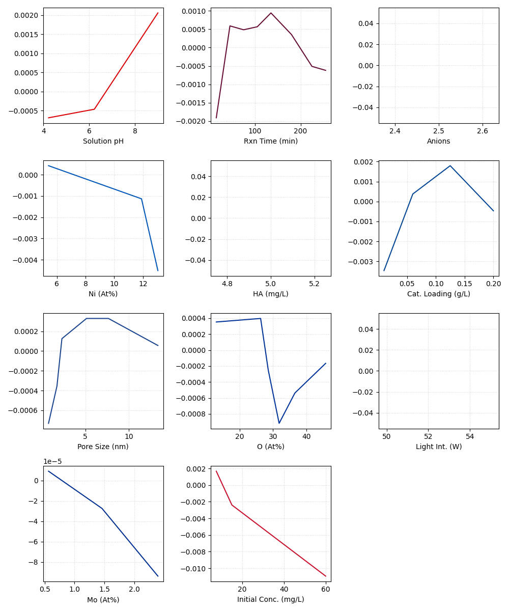
Partial Dependence Plot
pdp = PartialDependencePlot(
    model.predict,
    TrainX,
    num_points=20,
    feature_names=TrainX.columns.tolist(),
    show=False,
    save=False
)
mpl.rcParams.update(mpl.rcParamsDefault)
colors = ["#DB0007", "#670E36", "#e30613", "#0057B8", "#6C1D45",
          "#034694", "#1B458F", "#003399", "#FFCD00", "#003090",
          "#C8102E", "#6CABDD", "#DA291C", "#241F20", "#00A650",
          "#D71920", "#132257", "#ED2127", "#7A263A", "#FDB913",
          "#DB0007", "#670E36", "#e30613", "#0057B8", "#6C1D45",
          "#034694", "#1B458F", "#003399", "#FFCD00", "#003090",
          ]

f, axes = create_subplots(TrainX.shape[1], figsize=(10, 12))

for ax, feature, clr in zip(axes.flat, TrainX.columns, colors):

    pdp_vals, ice_vals = pdp.calc_pdp_1dim(TrainX.values, feature)

    ax = pdp.plot_pdp_1dim(pdp_vals, ice_vals, TrainX.values,
                            feature,
                            pdp_line_kws={
                                'color': clr, 'zorder': 3},
                            ice_color="gray",
                            ice_lines_kws=dict(zorder=2, alpha=0.15),
                            ax=ax,
                            show=False,
                            )
    ax.set_xlabel(LABEL_MAP.get(feature, feature))
    ax.set_ylabel(f"E[f(x) | " + feature + "]")
if SAVE:
    plt.savefig("results/figures/pdp.png", dpi=600, bbox_inches="tight")
plt.tight_layout()
plt.show()

Accumulated Local Effects
class MyModel:
    def predict(self, X):
        return model.predict(X).reshape(-1,)

f, axes = create_subplots(TrainX.shape[1], figsize=(10, 12))

for ax, feature, clr in zip(axes.flat, TrainX.columns, colors):
    plot_ale(MyModel().predict, TrainX, feature,
             ax=ax, show=False, color=clr, )

plt.tight_layout()
plt.show()
All Features model interpretation
For the sake of comparison, we also show interpretation of model which uses all features as input.
set_rcParams()

data, encoders = prepare_data(outputs="k")

print(data.shape)
(1527, 35)
input_features = data.columns.tolist()[0:-1]
output_features = data.columns.tolist()[-1:]

TrainX, TestX, TrainY, TestY = TrainTestSplit(seed=313).split_by_random(
    data[input_features],
    data[output_features]
)

print(TrainX.shape, TrainY.shape, TestX.shape, TestY.shape)


model = Model(
    model = "DecisionTreeRegressor",
    input_features=input_features,
    output_features=output_features,
    verbosity=-1,
)

model.fit(TrainX, TrainY.values)
(1068, 34) (1068, 1) (459, 34) (459, 1)
train_p = model.predict(TrainX, process_results=False)
test_p = model.predict(TestX, process_results=False)
Average prediction on training data
print(train_p.mean())
0.0069402254388336235
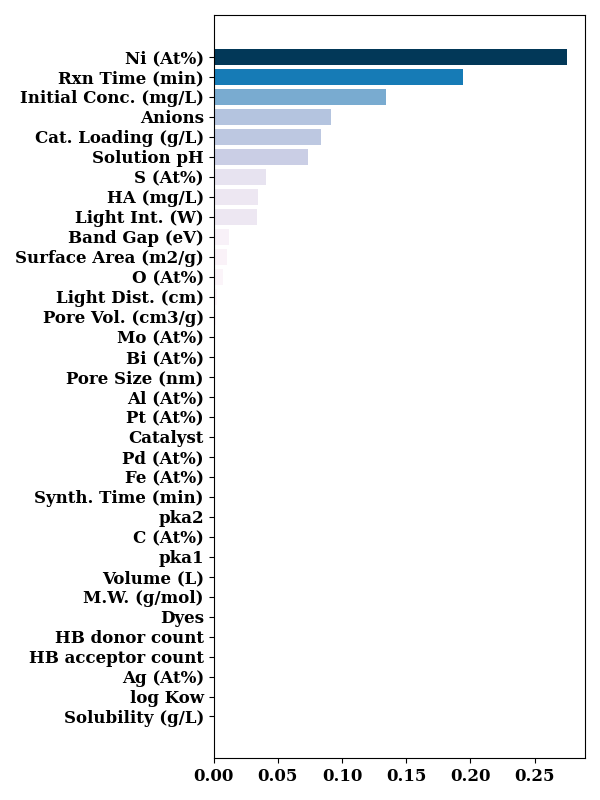
default feature importance from decision tree
print(model._model.feature_importances_)
[3.81006042e-05 1.73386029e-06 1.19712970e-02 0.00000000e+00
 7.23370042e-03 1.99232034e-05 3.97314739e-04 2.75412342e-01
 1.25751993e-03 4.10362230e-02 9.97703911e-04 0.00000000e+00
 2.34364582e-05 2.25969210e-04 1.03530578e-02 2.14975624e-03
 5.75046118e-04 0.00000000e+00 8.39858878e-02 3.36541611e-02
 2.61657725e-03 1.93957659e-01 0.00000000e+00 0.00000000e+00
 0.00000000e+00 0.00000000e+00 0.00000000e+00 0.00000000e+00
 0.00000000e+00 0.00000000e+00 1.34414955e-01 7.38624495e-02
 3.42792786e-02 9.15359069e-02]
fig, ax = plt.subplots(figsize=(6, 8))
bar_chart(model._model.feature_importances_,
          [LABEL_MAP[n] if n in LABEL_MAP else n for n in model.input_features],
          sort=True,
          show=False,
          ax=ax)
plt.tight_layout()
plt.show()
SHAP all features
exp = shap.TreeExplainer(model=model._model,
                         data=TrainX,
                         feature_names=input_features)

print(exp.expected_value)
0.00671328508398034
shap_values = exp.shap_values(TrainX, TrainY)

summary_plot(shap_values,
    TrainX,
             max_display=34,
feature_names=[LABEL_MAP[n] if n in LABEL_MAP else n for n in input_features],
    show=False)
if SAVE:
    plt.savefig("results/figures/shap_summary_all.png", dpi=600, bbox_inches="tight")
plt.tight_layout()
plt.show()

# sv_bar = np.mean(np.abs(shap_values), axis=0)

# classes, colors, colors_ = make_classes(exp)

# df_with_classes = pd.DataFrame({'features': exp.feature_names,
#                    'classes': classes,
#                    'mean_shap': sv_bar})

# print(df_with_classes)

# # %%
# f, ax = plt.subplots(figsize=(7,9))
# ax = bar_chart(
#     sv_bar,
#     [LABEL_MAP[n] if n in LABEL_MAP else n for n in exp.feature_names],
#     bar_labels=np.round(sv_bar, 4),
#     bar_label_kws={'label_type':'edge',
#                    'fontsize': 10,
#                    'weight': 'bold',
#                    "fmt": '%.4f',
#                    'padding': 1.5
#                    },
#     show=False,
#     sort=True,
#     color=colors_,
#     ax = ax
# )
# ax.spines[['top', 'right']].set_visible(False)
# ax.set_xlabel(xlabel='mean(|SHAP value|)')
# ax.set_xticklabels(ax.get_xticks().astype(float))
# ax.set_yticklabels(ax.get_yticklabels())

# labels = df_with_classes['classes'].unique()
# handles = [plt.Rectangle((0,0),1,1,
#                          color=colors[l]) for l in labels]
# plt.legend(handles, labels, loc='lower right')
# ax.xaxis.set_major_locator(plt.MaxNLocator(4))
# if SAVE:
#     plt.savefig("results/figures/shap_bar_all.png", dpi=600, bbox_inches="tight")
# plt.tight_layout()
# plt.show()

# # %%

# seg_colors = (colors.values())
# # Change the saturation of seg_colors to 70% for the interior segments
# rgb = mcolors.to_rgba_array(seg_colors)[:,:-1]
# hsv = mcolors.rgb_to_hsv(rgb)
# hsv[:,1] = 0.7 * hsv[:, 1]
# interior_colors = mcolors.hsv_to_rgb(hsv)

# fractions = np.array([
# df_with_classes.loc[df_with_classes['classes']=='Experimental Conditions']['mean_shap'].sum(),
# df_with_classes.loc[df_with_classes['classes']=='Physicochemical Properties']['mean_shap'].sum(),
# df_with_classes.loc[df_with_classes['classes']=='Atomic Composition']['mean_shap'].sum(),
# ])

# dye_frac = df_with_classes.loc[df_with_classes['classes']=='Dye Properties']['mean_shap'].sum()
# labels = ['Experimental \nConditions', 'Physicochemical \nProperties',
#                'Atomic \nComposition']

# if dye_frac > 0.0:
#     fractions = np.array(fractions.tolist().append(dye_frac))
#     labels.append('Dye Properties')

# fractions /=fractions.sum()

# _, texts= pie(fractions=fractions,
#     colors=seg_colors,
#     labels=labels,
#     wedgeprops=dict(edgecolor="w", width=0.03), radius=1,
#     autopct=None,
#     textprops = dict(fontsize=12),
#     startangle=90, counterclock=False, show=False)
# texts[0].set_fontsize(12)
# _, texts, autotexts = pie(fractions=fractions,
#     colors=interior_colors,
#        autopct='%1.0f%%',
#     textprops = dict(fontsize=24),
#     wedgeprops=dict(edgecolor="w"), radius=1-2*0.03,
#     startangle=90, counterclock=False, ax=plt.gca(), show=False)
# texts[0].set_fontsize(12)
# if SAVE:
#     plt.savefig("results/figures/shap_pie_all.png", dpi=600, bbox_inches="tight")
# plt.tight_layout()
# plt.show()
Total running time of the script: (0 minutes 56.549 seconds)